Example: “Lotka-Volterra” Equations
Scope
This notebook introduces the input format of yaml2sbml and showcases the Python interface of the tool. Furthermore, this notebook demonstrates the simulation of an SBML model using AMICI and parameter estimation from PEtab using pyPESTO.
Equations
The “Lotka-Volterra” Equations are given by
Here \(x_1\) denotes the number of a prey and \(x_2\) the number of a predator species and \(\alpha, \beta, \gamma, \delta\) are positive parameters describing the birth/death and interactions of the two species.
YAML file for model simulation in SBML:
The states \(x_1\) and \(x_2\), as well as their initial values and dynamics are defined in the odes: section:
odes:
    - stateId: x_1
      rightHandSide: alpha * x_1 - beta * x_1 * x_2
      initialValue: 2

    - stateId: x_2
      rightHandSide: delta * x_1 * x_2 - gamma * x_2
      initialValue: 2
Furthermore, the parameters together with their values are defined in the parameters: section:
parameters:
    - parameterId: alpha
      nominalValue: 2

    - parameterId: beta
      nominalValue: 4

   ...
The full file is given in Lotka_Volterra_basic.yml.
Format validation of the YAML model:
The YAML model can be validated by the yaml2sbml package via:
[1]:
import yaml2sbml

yaml_file_basic = 'Lotka_Volterra_basic.yml'
yaml2sbml.validate_yaml(yaml_dir=yaml_file_basic)
YAML file is valid ✅
Conversion to SBML for model simulation:
We now want to convert the YAML file into a SBML file. Within Python this is possible via:
[2]:
import yaml2sbml

sbml_output_file = 'Lotka_Volterra_basic.xml'
yaml2sbml.yaml2sbml(yaml_file_basic, sbml_output_file)
We will now use the SBML simulator AMICI to simulate the ODEs. First AMICI generates the models’ C++ code.
[3]:
%%capture

import amici
import amici.plotting

model_name = 'Lotka_Volterra'
model_output_dir = 'Lotka_Volterra_AMICI'

sbml_importer = amici.SbmlImporter(sbml_output_file)
sbml_importer.sbml2amici(model_name,
                         model_output_dir)
Then we can reload and simulate the compiled model.
[4]:
%%capture

import os
import sys
import importlib
import numpy as np

# import model
sys.path.insert(0, os.path.abspath(model_output_dir))
model_module = importlib.import_module(model_name)

# create model + solver instance
model = model_module.getModel()
solver = model.getSolver()

# Define time points and run simulation using default model parameters/solver options
model.setTimepoints(np.linspace(0, 20, 201))
rdata = amici.runAmiciSimulation(model, solver)
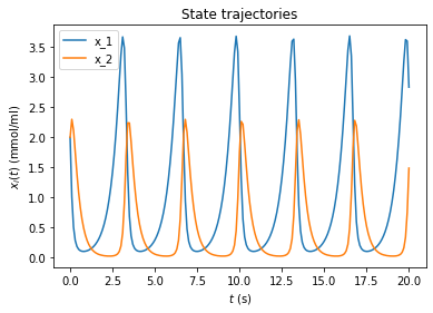
[5]:
# plot trajectories
amici.plotting.plotStateTrajectories(rdata, model=model)
Conversion to PEtab for parameter fitting:
In order to obtain valid PEtab tables, we need to extend the .yml file. The extended .yml file is given as Lotka_Volterra_PEtab.yml.
Parameters:
The parameters: section can be extended to store parameter bounds, transformations, … This information is written to the PEtab parameter table.
parameters:
    - parameterId: alpha
      nominalValue: 2
      parameterScale: log10
      lowerBound: 0.01
      upperBound: 100
      estimate: 1

   ...
(Note: PEtab measurement tables are outside of the scope of yaml2sbml. Hence a predefined measurement table for this example is given under ./Lotka_Volterra_PEtab/measurement_table.tsv.)
Observables:
The observables: section allows to specify the mapping of system state to measurement and the measurement noise. This information is written in the PEtab observable table.
observables:
    - observableId: prey_measured
      observableFormula: log10(x_1)
      observableTransformation: lin
      noiseFormula: 1
      noiseDistribution: normal
Conditions:
The conditions: section allows to specify different experimental setups. This information is written in the PEtab condition table. This example only defines the trivial condition table, consisting of only one experimental setup.
conditions:
    - conditionId: condition1
yaml2petab:
We want to create the corresponding PEtab tables for the model in Lotka_Volterra_PEtab.yml. Since the definition of PEtab measurement tables is outside of the scope of yaml2sbml, a predefined measurement table is given under ./Lotka_Volterra_PEtab/measurement_table.tsv.
[6]:
yaml_file_petab = 'Lotka_Volterra_PEtab.yml'
PEtab_dir = './Lotka_Volterra_PEtab/'
PEtab_yaml_name = 'problem.yml'
measurement_table_name = 'measurement_table.tsv'
model_name = 'Lotka_Volterra_with_observables'

yaml2sbml.yaml2petab(yaml_file_petab,
                     PEtab_dir,
                     model_name,
                     PEtab_yaml_name,
                     measurement_table_name)
yaml2petab created the PEtab files. In the following we show how to import and fit a PEtab problem in pyPESTO.
[7]:
%%capture
import pypesto
import pypesto.petab
import pypesto.optimize as optimize
import pypesto.visualize as visualize

# import PEtab problem
importer = pypesto.petab.PetabImporter.from_yaml(os.path.join(PEtab_dir, PEtab_yaml_name),
                                                 model_name=model_name)
problem = importer.create_problem()
Perform the fitting:
[8]:
%%capture
# perform optimization
optimizer = optimize.ScipyOptimizer()
result = optimize.minimize(problem,
                           optimizer=optimizer,
                           n_starts=10)
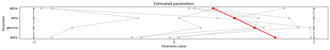
Next we want to visualize the results using parallel coordinate plots.
[9]:
visualize.parameters(result)
[9]:
<matplotlib.axes._subplots.AxesSubplot at 0x7ff95ff93d30>